Welcome to GSTools

Get in Touch!

Youtube Tutorial on GSTools

Purpose

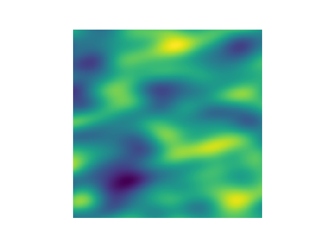
GSTools provides geostatistical tools for various purposes:

• random field generation, including periodic boundaries


• simple, ordinary, universal and external drift kriging


• conditioned field generation


• incompressible random vector field generation


• (automated) variogram estimation and fitting


• directional variogram estimation and modelling


• data normalization and transformation


• many readily provided and even user-defined covariance models


• metric spatio-temporal modelling


• plurigaussian field simulations (PGS)


• plotting and exporting routines

Installation

conda

GSTools can be installed via conda on Linux, Mac, and Windows.

Install the package by typing the following command in a command terminal:

conda install gstools

In case conda forge is not set up for your system yet, see the easy to follow

instructions on conda forge. Using conda, the parallelized

version of GSTools should be installed.

pip

GSTools can be installed via pip on Linux, Mac, and Windows.

On Windows you can install WinPython to get Python and pip

running. Install the package by typing the following command in a command terminal:

pip install gstools

To install the latest development version via pip, see the

documentation.

One thing to point out is that this way, the non-parallel version of GSTools

is installed. In case you want the parallel version, follow these easy

steps.

Citation

If you are using GSTools in your publication please cite our paper:

Müller, S., Schüler, L., Zech, A., and Heße, F.:

GSTools v1.3: a toolbox for geostatistical modelling in Python,

Geosci. Model Dev., 15, 3161–3182, https://doi.org/10.5194/gmd-15-3161-2022, 2022.

You can cite the Zenodo code publication of GSTools by:

Sebastian Müller & Lennart Schüler. GeoStat-Framework/GSTools. Zenodo. https://doi.org/10.5281/zenodo.1313628

If you want to cite a specific version, have a look at the Zenodo site.

Documentation for GSTools

You can find the documentation under geostat-framework.readthedocs.io.

Tutorials and Examples

The documentation also includes some tutorials, showing the most important use cases of GSTools, which are

• Random Field Generation


• The Covariance Model


• Variogram Estimation


• Random Vector Field Generation


• Kriging


• Conditioned random field generation


• Field transformations


• Geographic Coordinates


• Spatio-Temporal Modelling


• Normalizing Data


• Plurigaussian Field Generation (PGS)


• Miscellaneous examples

The associated python scripts are provided in the examples folder.

Spatial Random Field Generation

The core of this library is the generation of spatial random fields. These fields are generated using the randomisation method, described by Heße et al. 2014.

Examples

Gaussian Covariance Model

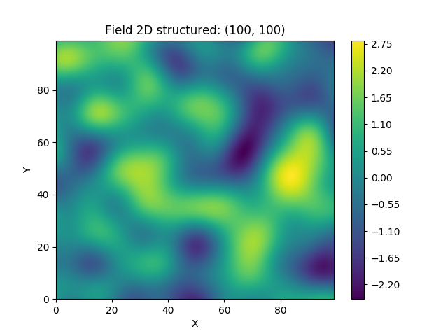
This is an example of how to generate a 2 dimensional spatial random field with a gaussian covariance model.

import gstools as gs
# structured field with a size 100x100 and a grid-size of 1x1
x = y = range(100)
model = gs.Gaussian(dim=2, var=1, len_scale=10)
srf = gs.SRF(model)
srf((x, y), mesh_type='structured')
srf.plot()

GSTools also provides support for geographic coordinates.

This works perfectly well with cartopy.

import matplotlib.pyplot as plt
import cartopy.crs as ccrs
import gstools as gs
# define a structured field by latitude and longitude
lat = lon = range(-80, 81)
model = gs.Gaussian(latlon=True, len_scale=777, geo_scale=gs.KM_SCALE)
srf = gs.SRF(model, seed=12345)
field = srf.structured((lat, lon))
# Orthographic plotting with cartopy
ax = plt.subplot(projection=ccrs.Orthographic(-45, 45))
cont = ax.contourf(lon, lat, field, transform=ccrs.PlateCarree())
ax.coastlines()
ax.set_global()
plt.colorbar(cont)

A similar example but for a three dimensional field is exported to a VTK file, which can be visualized with ParaView or PyVista in Python:

import gstools as gs
# structured field with a size 100x100x100 and a grid-size of 1x1x1
x = y = z = range(100)
model = gs.Gaussian(dim=3, len_scale=[16, 8, 4], angles=(0.8, 0.4, 0.2))
srf = gs.SRF(model)
srf((x, y, z), mesh_type='structured')
srf.vtk_export('3d_field') # Save to a VTK file for ParaView


mesh = srf.to_pyvista() # Create a PyVista mesh for plotting in Python
mesh.contour(isosurfaces=8).plot()

Estimating and Fitting Variograms

The spatial structure of a field can be analyzed with the variogram, which contains the same information as the covariance function.

All covariance models can be used to fit given variogram data by a simple interface.

Example

This is an example of how to estimate the variogram of a 2 dimensional unstructured field and estimate the parameters of the covariance

model again.

import numpy as np
import gstools as gs
# generate a synthetic field with an exponential model
x = np.random.RandomState(19970221).rand(1000) * 100.
y = np.random.RandomState(20011012).rand(1000) * 100.
model = gs.Exponential(dim=2, var=2, len_scale=8)
srf = gs.SRF(model, mean=0, seed=19970221)
field = srf((x, y))
# estimate the variogram of the field
bin_center, gamma = gs.vario_estimate((x, y), field)
# fit the variogram with a stable model. (no nugget fitted)
fit_model = gs.Stable(dim=2)
fit_model.fit_variogram(bin_center, gamma, nugget=False)
# output
ax = fit_model.plot(x_max=max(bin_center))
ax.scatter(bin_center, gamma)
print(fit_model)

Which gives:

Stable(dim=2, var=1.85, len_scale=7.42, nugget=0.0, anis=[1.0], angles=[0.0], alpha=1.09)

Kriging and Conditioned Random Fields

An important part of geostatistics is Kriging and conditioning spatial random

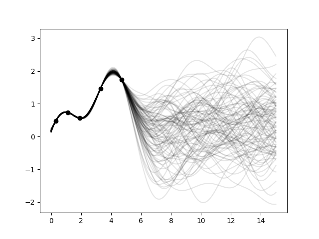
fields to measurements. With conditioned random fields, an ensemble of field realizations with their variability depending on the proximity of the measurements can be generated.

Example

For better visualization, we will condition a 1d field to a few "measurements", generate 100 realizations and plot them:

import numpy as np
import matplotlib.pyplot as plt
import gstools as gs


# conditions
cond_pos = [0.3, 1.9, 1.1, 3.3, 4.7]
cond_val = [0.47, 0.56, 0.74, 1.47, 1.74]

# conditioned spatial random field class
model = gs.Gaussian(dim=1, var=0.5, len_scale=2)
krige = gs.krige.Ordinary(model, cond_pos, cond_val)
cond_srf = gs.CondSRF(krige)
# same output positions for all ensemble members
grid_pos = np.linspace(0.0, 15.0, 151)
cond_srf.set_pos(grid_pos)

# seeded ensemble generation
seed = gs.random.MasterRNG(20170519)
for i in range(100):
    field = cond_srf(seed=seed(), store=f"field_{i}")
    plt.plot(grid_pos, field, color="k", alpha=0.1)
plt.scatter(cond_pos, cond_val, color="k")
plt.show()

User Defined Covariance Models

One of the core-features of GSTools is the powerful

CovModel

class, which allows to easy define covariance models by the user.

Example

Here we re-implement the Gaussian covariance model by defining just a

correlation function, which takes a non-dimensional distance h = r/l:

import numpy as np
import gstools as gs
# use CovModel as the base-class
class Gau(gs.CovModel):
    def cor(self, h):
        return np.exp(-h**2)

And that's it! With Gau you now have a fully working covariance model,

which you could use for field generation or variogram fitting as shown above.

Have a look at the documentation for further information on incorporating

optional parameters and optimizations.

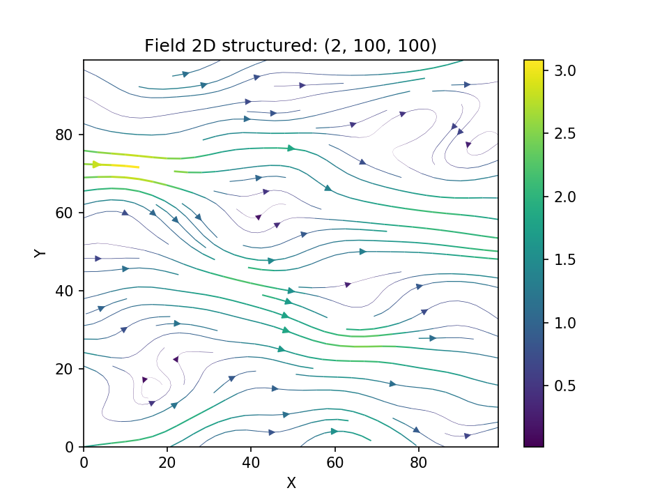
Incompressible Vector Field Generation

Using the original Kraichnan method, incompressible random

spatial vector fields can be generated.

Example

import numpy as np
import gstools as gs
x = np.arange(100)
y = np.arange(100)
model = gs.Gaussian(dim=2, var=1, len_scale=10)
srf = gs.SRF(model, generator='VectorField', seed=19841203)
srf((x, y), mesh_type='structured')
srf.plot()

yielding

Plurigaussian Field Simulation (PGS)

With PGS, more complex categorical (or discrete) fields can be created.

Example

import gstools as gs
import numpy as np
import matplotlib.pyplot as plt


N = [180, 140]

x, y = range(N[0]), range(N[1])

# we need 2 SRFs
model = gs.Gaussian(dim=2, var=1, len_scale=5)
srf = gs.SRF(model)
field1 = srf.structured([x, y], seed=20170519)
field2 = srf.structured([x, y], seed=19970221)

# with `lithotypes`, we prescribe the categorical data and its relations
# here, we use 2 categories separated by a rectangle.
rect = [40, 32]
lithotypes = np.zeros(N)
lithotypes[
    N[0] // 2 - rect[0] // 2 : N[0] // 2 + rect[0] // 2,
    N[1] // 2 - rect[1] // 2 : N[1] // 2 + rect[1] // 2,
] = 1

pgs = gs.PGS(2, [field1, field2])
P = pgs(lithotypes)

fig, axs = plt.subplots(1, 2)
axs[0].imshow(lithotypes, cmap="copper")
axs[1].imshow(P, cmap="copper")
plt.show()

VTK/PyVista Export

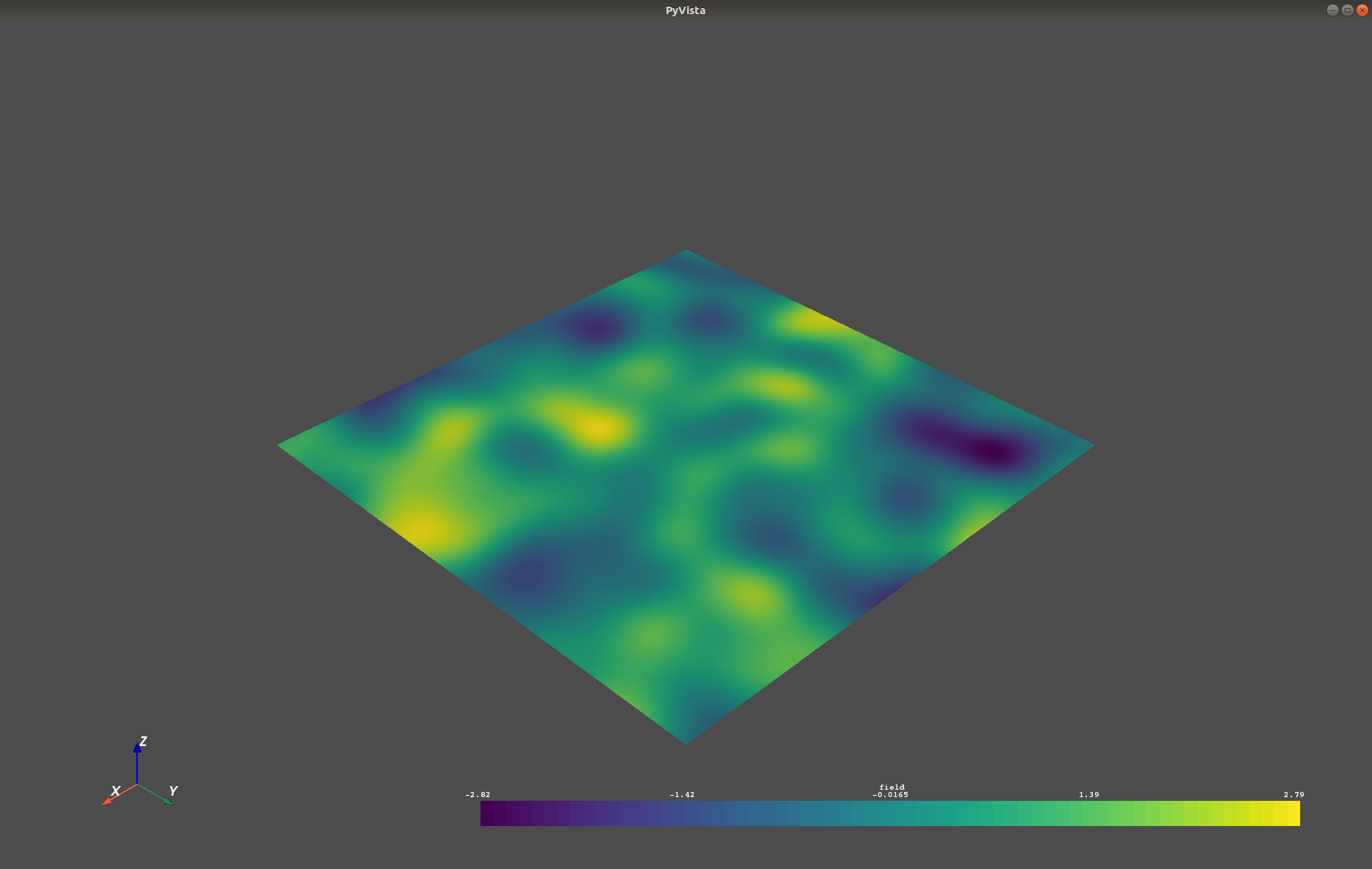
After you have created a field, you may want to save it to file, so we provide

a handy VTK export routine using the .vtk_export() or you could

create a VTK/PyVista dataset for use in Python with to .to_pyvista() method:

import gstools as gs
x = y = range(100)
model = gs.Gaussian(dim=2, var=1, len_scale=10)
srf = gs.SRF(model)
srf((x, y), mesh_type='structured')
srf.vtk_export("field") # Saves to a VTK file
mesh = srf.to_pyvista() # Create a VTK/PyVista dataset in memory
mesh.plot()

Which gives a RectilinearGrid VTK file field.vtr or creates a PyVista mesh

in memory for immediate 3D plotting in Python.

Requirements:

• NumPy >= 1.20.0


• SciPy >= 1.1.0


• hankel >= 1.0.0


• emcee >= 3.0.0


• pyevtk >= 1.1.1


• meshio >= 5.1.0

Optional

• GSTools-Core >= 0.2.0


• matplotlib


• pyvista

Contact

You can contact us via info@geostat-framework.org.

License

LGPLv3 © 2018-2025